什么是扩散模型

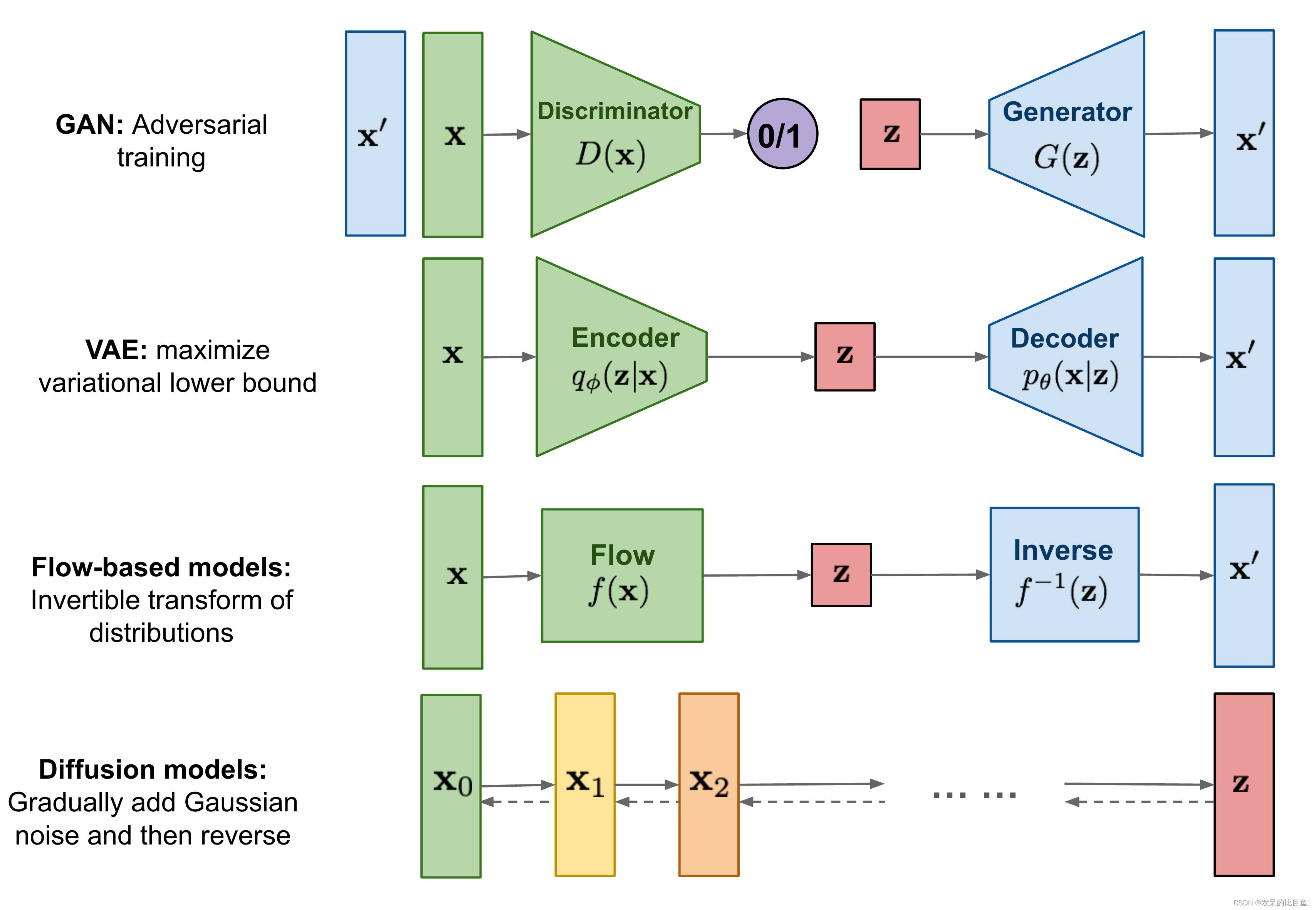
关于GAN、VAE和基于Flow模型的生成模型。在生成高质量样本方面取得了巨大成功，但每个都有其自身的局限性。GAN 模型因其对抗性训练性质而以潜在的不稳定训练和较少的生成多样性而闻名。VAE 依赖于替代损失。流模型必须使用专门的架构来构建可逆变换。

扩散模型的灵感来自于非平衡热力学。他们定义了一个扩散步骤的马尔可夫链，慢慢地向数据中添加随机噪声，然后学习反向扩散过程，从噪声中构建所需的数据样本。与VAE或流动模型不同，扩散模型的学习过程是固定的，潜在变量具有高维性(与原始数据相同)。

什么是扩散模型

人们提出了几种基于扩散的生成模型，其中包括扩散概率模型(Sohl-Dickstein et al., 2015)、噪声条件评分网络(NCSN;Yang & Ermon, 2019)和去噪扩散概率模型(DDPM; Hoet al.，2020)。

向前扩散过程

给定一个从真实数据分布中抽样的数据点${\mathbf{x}}_0\sim q(\mathbf{x})$, 让我们定义一个正向扩散过程，在$T$步中向样本添加少量高斯噪声，产生一个噪声样本序列$x_1，，x_T$。步长大小由方差控制：{βt∈(0,1)}t=1T\{\beta_t \in (0, 1)\}_{t=1}^T{βt​∈(0,1)}t=1T​
$$q({\mathbf{x}}_t|{\mathbf{x}}_{t-1})=\mathcal{N}({\mathbf{x}}_t;\sqrt{1-{\beta }_t}{\mathbf{x}}_{t-1},{\beta }_t\mathbf{I})q({\mathbf{x}}_{1:T}|{\mathbf{x}}_0)=\prod _{t=1}^{T}q({\mathbf{x}}_t|{\mathbf{x}}_{t-1})$$

随着步长$t$的增大，数据样本$x_0$逐渐失去其可区分的特征。最终当$T$时，$x_T$等价于各向同性高斯分布。

上述过程的一个很好的特性是，我们可以使用重新参数化技巧在任意时间步$t$以封闭形式对$x_t$进行采样。令${\alpha }_t=1-{\beta }_t$ 和${\bar{\alpha }}_t={\prod }_{i=1}^T{\alpha }_i$

$$\begin{array}{rlr}{\mathbf{x}}_t& =\sqrt{{\alpha }_t}{\mathbf{x}}_{t-1}+\sqrt{1-{\alpha }_t}{\mathbf{z}}_{t-1}& \text{ ;where }{\mathbf{z}}_{t-1},{\mathbf{z}}_{t-2},\cdots \sim \mathcal{N}(0,\mathbf{I})\\ & =\sqrt{{\alpha }_t{\alpha }_{t-1}}{\mathbf{x}}_{t-2}+\sqrt{1-{\alpha }_t{\alpha }_{t-1}}{\bar{\mathbf{z}}}_{t-2}& \text{ ;where }{\bar{\mathbf{z}}}_{t-2}\text{ merges two Gaussians (*).}\\ & =\dots & \\ & =\sqrt{{\bar{\alpha }}_t}{\mathbf{x}}_0+\sqrt{1-{\bar{\alpha }}_t}\mathbf{z}& \\ q({\mathbf{x}}_t|{\mathbf{x}}_0)& =\mathcal{N}({\mathbf{x}}_t;\sqrt{{\bar{\alpha }}_t}{\mathbf{x}}_0,(1-{\bar{\alpha }}_t)\mathbf{I})& \end{array}$$

(*)回想一下，当我们合并两个方差不同的高斯函数时$\mathcal{N}(0,{\sigma }_1^2\mathbf{I})$和$\mathcal{N}(\mathbf{0}, \sigma_2^2\mathbf{I})
$，新的分布是$\mathcal{N}(\mathbf{0}, (\sigma_1^2 + \sigma_2^2)\mathbf{I})$,合并标准差是$\sqrt{(1 - \alpha_t) + \alpha_t (1-\alpha_{t-1})} = \sqrt{1 - \alpha_t\alpha_{t-1}}$

通常情况下，当样本噪音更大时，我们可以承担更大的更新步骤，所以${\beta }_1<{\beta }_2<\cdots <{\beta }_T$和${\bar{\alpha }}_1>\cdots >{\bar{\alpha }}_T$

与随机梯度Langevin动力学关系

Langevin 动力学是一个来自物理学的概念，用于分子系统的统计建模。结合随机梯度下降，随机梯度Langevin动力学(Welling & Teh 2011)仅使用马尔可夫更新链中的梯度$\nabla xlogp(x)$就可以从概率密度$p(x)$中产生样本:
$${\mathbf{x}}_t={\mathbf{x}}_{t-1}+\frac{ϵ}{2}{\nabla }_{\mathbf{x}}\log p({\mathbf{x}}_{t-1})+\sqrt{ϵ}{\mathbf{z}}_t,\text{where }{\mathbf{z}}_t\sim \mathcal{N}(0,\mathbf{I})$$

其中， $ϵ$是步长。当$T\to \infty ,ϵ\to 0$时,$X^T$等于真实概率密度$p(x)$。
与标准SGD相比，随机梯度Langevin动力学在参数更新中注入了高斯噪声，避免了陷入局部极小值。

反向扩散过程

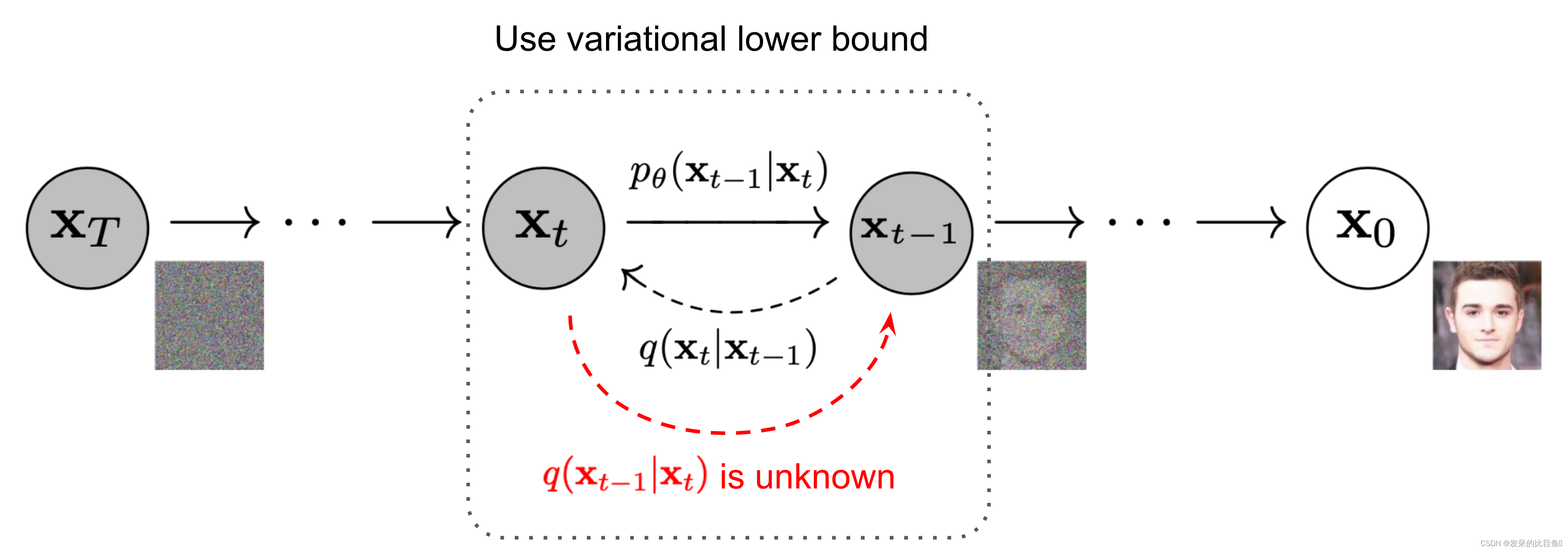
如果我们可以逆转上述过程，并从$q({\mathbf{x}}_{t-1}|{\mathbf{x}}_t)$采样，我们将能够从高斯噪声输入${\mathbf{x}}_T\sim \mathcal{N}(0,\mathbf{I})$重建真实的样本。注意，如果${\beta }_t$足够小，$q({\mathbf{x}}_{t-1}|{\mathbf{x}}_t)$也将是高斯分布。不幸的是，我们不能轻易地估计$q({\mathbf{x}}_{t-1}|{\mathbf{x}}_t)$，因为它需要使用整个数据集，因此我们需要学习一个模型$p_{\theta }$来近似这些条件概率，以便运行反向扩散过程。
$$p_{\theta }({\mathbf{x}}_{0:T})=p({\mathbf{x}}_T)\prod _{t=1}^T{p}_{\theta }({\mathbf{x}}_{t-1}|{\mathbf{x}}_t)p_{\theta }({\mathbf{x}}_{t-1}|{\mathbf{x}}_t)=\mathcal{N}({\mathbf{x}}_{t-1};{\mathbf{\mu }}_{\theta }({\mathbf{x}}_t,t),{\mathbf{\Sigma }}_{\theta }({\mathbf{x}}_t,t))$$

值得注意的是，当条件为$x_0$时，反向条件概率是
$$q({\mathbf{x}}_{t-1}|{\mathbf{x}}_t,{\mathbf{x}}_0)=\mathcal{N}({\mathbf{x}}_{t-1};\tilde{\mathbf{\mu }}({\mathbf{x}}_t,{\mathbf{x}}_0),{\tilde{\beta }}_t\mathbf{I})$$

也就是说，给定$x_t$，和$x_0$，我们是可以计算出$x_{t-1}$
注意：高斯分布的概率密度函数是$f(x)=\frac{1}{\sqrt{2\pi \sigma }}{e}^{-\frac{(x-\mu {)}^2}{2{\sigma }^2}}$

注意：$a{x}^2+bx=a(x+\frac{b}{2a}{)}^2+C$

使用贝叶斯规则，我们有
$$\begin{array}{rl}q({\mathbf{x}}_{t-1}|{\mathbf{x}}_t,{\mathbf{x}}_0)& =q({\mathbf{x}}_t|{\mathbf{x}}_{t-1},{\mathbf{x}}_0)\frac{q({\mathbf{x}}_{t-1}|{\mathbf{x}}_0)}{q({\mathbf{x}}_t|{\mathbf{x}}_0)}\\ & \propto \exp (-\frac{1}{2}(\frac{({\mathbf{x}}_t-\sqrt{{\alpha }_t}{\mathbf{x}}_{t-1}{)}^2}{{\beta }_t}+\frac{({\mathbf{x}}_{t-1}-\sqrt{{\bar{\alpha }}_{t-1}}{\mathbf{x}}_0{)}^2}{1-{\bar{\alpha }}_{t-1}}-\frac{({\mathbf{x}}_t-\sqrt{{\bar{\alpha }}_t}{\mathbf{x}}_0{)}^2}{1-{\bar{\alpha }}_t}\left)\right)\\ & =\exp (-\frac{1}{2}(\frac{{\mathbf{x}}_t^2-2\sqrt{{\alpha }_t}{\mathbf{x}}_t{\mathbf{x}}_{t-1}+{\alpha }_t{\mathbf{x}}_{t-1}^2}{{\beta }_t}+\frac{{\mathbf{x}}_{t-1}^2-2\sqrt{{\bar{\alpha }}_{t-1}}{\mathbf{x}}_0{\mathbf{x}}_{t-1}+{\bar{\alpha }}_{t-1}{\mathbf{x}}_0^2}{1-{\bar{\alpha }}_{t-1}}-\frac{({\mathbf{x}}_t-\sqrt{{\bar{\alpha }}_t}{\mathbf{x}}_0{)}^2}{1-{\bar{\alpha }}_t}\left)\right)\\ & =\exp (-\frac{1}{2}((\frac{{\alpha }_t}{{\beta }_t}+\frac{1}{1-{\bar{\alpha }}_{t-1}}){\mathbf{x}}_{t-1}^2-(\frac{2\sqrt{{\alpha }_t}}{{\beta }_t}{\mathbf{x}}_t+\frac{2\sqrt{{\bar{\alpha }}_{t-1}}}{1-{\bar{\alpha }}_{t-1}}{\mathbf{x}}_0){\mathbf{x}}_{t-1}+C({\mathbf{x}}_t,{\mathbf{x}}_0)\left)\right)\end{array}$$

其中，$C({\mathbf{x}}_t,{\mathbf{x}}_0)$ 是一个不涉及$x_{t-1}$的函数，细节略。按照标准的高斯密度函数，均值和方差可以如下参数化(${\alpha }_t=1-{\beta }_t$, ${\bar{\alpha }}_t={\prod }_{i=1}^T{\alpha }_i$):

$$\begin{array}{rl}{\tilde{\beta }}_t& =1/(\frac{{\alpha }_t}{{\beta }_t}+\frac{1}{1-{\bar{\alpha }}_{t-1}})=1/(\frac{{\alpha }_t-{\bar{\alpha }}_t+{\beta }_t}{{\beta }_t(1-{\bar{\alpha }}_{t-1})})=\frac{1-{\bar{\alpha }}_{t-1}}{1-{\bar{\alpha }}_t}\cdot {\beta }_t\\ {\tilde{\mathbf{\mu }}}_t({\mathbf{x}}_t,{\mathbf{x}}_0)& =(\frac{\sqrt{{\alpha }_t}}{{\beta }_t}{\mathbf{x}}_t+\frac{\sqrt{{\bar{\alpha }}_{t-1}}}{1-{\bar{\alpha }}_{t-1}}{\mathbf{x}}_0)/(\frac{{\alpha }_t}{{\beta }_t}+\frac{1}{1-{\bar{\alpha }}_{t-1}})\\ & =(\frac{\sqrt{{\alpha }_t}}{{\beta }_t}{\mathbf{x}}_t+\frac{\sqrt{{\bar{\alpha }}_{t-1}}}{1-{\bar{\alpha }}_{t-1}}{\mathbf{x}}_0)\frac{1-{\bar{\alpha }}_{t-1}}{1-{\bar{\alpha }}_t}\cdot {\beta }_t\\ & =\frac{\sqrt{{\alpha }_t}(1-{\bar{\alpha }}_{t-1})}{1-{\bar{\alpha }}_t}{\mathbf{x}}_t+\frac{\sqrt{{\bar{\alpha }}_{t-1}}{\beta }_t}{1-{\bar{\alpha }}_t}{\mathbf{x}}_0\end{array}$$

由于这个很好的性质，我们可以表示${\mathbf{x}}_0=\frac{1}{\sqrt{{\bar{\alpha }}_t}}({\mathbf{x}}_t-\sqrt{1-{\bar{\alpha }}_t}{\mathbf{z}}_t)$，代入上述方程得到
$$\begin{array}{rl}{\tilde{\mathbf{\mu }}}_t& =\frac{\sqrt{{\alpha }_t}(1-{\bar{\alpha }}_{t-1})}{1-{\bar{\alpha }}_t}{\mathbf{x}}_t+\frac{\sqrt{{\bar{\alpha }}_{t-1}}{\beta }_t}{1-{\bar{\alpha }}_t}\frac{1}{\sqrt{{\bar{\alpha }}_t}}({\mathbf{x}}_t-\sqrt{1-{\bar{\alpha }}_t}{\mathbf{z}}_t)\\ & =\frac{1}{\sqrt{{\alpha }_t}}({\mathbf{x}}_t-\frac{{\beta }_t}{\sqrt{1-{\bar{\alpha }}_t}}{\mathbf{z}}_t)\end{array}$$

在如图2中。这样的设置与VAE非常相似，因此我们可以使用变分下界来优化负对数似然。

$$\begin{array}{rl}\log p_{\theta }({\mathbf{x}}_0)& \le -\log p_{\theta }({\mathbf{x}}_0)+D_{\text{KL}}(q({\mathbf{x}}_{1:T}|{\mathbf{x}}_0)\Vert p_{\theta }({\mathbf{x}}_{1:T}|{\mathbf{x}}_0))\\ & =-\log p_{\theta }({\mathbf{x}}_0)+{\mathbb{E}}_{{\mathbf{x}}_{1:T}\sim q({\mathbf{x}}_{1:T}|{\mathbf{x}}_0)}\left[\log \frac{q({\mathbf{x}}_{1:T}|{\mathbf{x}}_0)}{p_{\theta }({\mathbf{x}}_{0:T})/p_{\theta }({\mathbf{x}}_0)}\right]\\ & =-\log p_{\theta }({\mathbf{x}}_0)+{\mathbb{E}}_q[\log \frac{q({\mathbf{x}}_{1:T}|{\mathbf{x}}_0)}{p_{\theta }({\mathbf{x}}_{0:T})}+\log p_{\theta }({\mathbf{x}}_0)]\\ & ={\mathbb{E}}_q\left[\log \frac{q({\mathbf{x}}_{1:T}|{\mathbf{x}}_0)}{p_{\theta }({\mathbf{x}}_{0:T})}\right]\\ \text{Let }{L}_{\text{VLB}}& ={\mathbb{E}}_{q({\mathbf{x}}_{0:T})}\left[\log \frac{q({\mathbf{x}}_{1:T}|{\mathbf{x}}_0)}{p_{\theta }({\mathbf{x}}_{0:T})}\right]\ge -{\mathbb{E}}_{q({\mathbf{x}}_0)}\log p_{\theta }({\mathbf{x}}_0)\end{array}$$

使用詹森不等式也可以直接得到相同的结果。假设我们想要最小化交叉熵作为学习目标:
$$\begin{array}{rl}{L}_{\text{CE}}& =-{\mathbb{E}}_{q({\mathbf{x}}_0)}\log p_{\theta }({\mathbf{x}}_0)\\ & =-{\mathbb{E}}_{q({\mathbf{x}}_0)}\log (\int p_{\theta }({\mathbf{x}}_{0:T})d{\mathbf{x}}_{1:T})\\ & =-{\mathbb{E}}_{q({\mathbf{x}}_0)}\log (\int q({\mathbf{x}}_{1:T}|{\mathbf{x}}_0)\frac{p_{\theta }({\mathbf{x}}_{0:T})}{q({\mathbf{x}}_{1:T}|{\mathbf{x}}_0)}d{\mathbf{x}}_{1:T})\\ & =-{\mathbb{E}}_{q({\mathbf{x}}_0)}\log \left({\mathbb{E}}_{q({\mathbf{x}}_{1:T}|{\mathbf{x}}_0)}\frac{p_{\theta }({\mathbf{x}}_{0:T})}{q({\mathbf{x}}_{1:T}|{\mathbf{x}}_0)}\right)\\ & \le -{\mathbb{E}}_{q({\mathbf{x}}_{0:T})}\log \frac{p_{\theta }({\mathbf{x}}_{0:T})}{q({\mathbf{x}}_{1:T}|{\mathbf{x}}_0)}\\ & ={\mathbb{E}}_{q({\mathbf{x}}_{0:T})}\left[\log \frac{q({\mathbf{x}}_{1:T}|{\mathbf{x}}_0)}{p_{\theta }({\mathbf{x}}_{0:T})}\right]=L_{\text{VLB}}\end{array}$$

为了将方程中的每一项转化为可解析计算，目标可以进一步改写为几个KL-散度和熵项的组合(Sohl-Dickstein et al., 2015)
$$\begin{array}{rl}{L}_{\text{VLB}}& ={\mathbb{E}}_{q({\mathbf{x}}_{0:T})}\left[\log \frac{q({\mathbf{x}}_{1:T}|{\mathbf{x}}_0)}{p_{\theta }({\mathbf{x}}_{0:T})}\right]\\ & ={\mathbb{E}}_q\left[\log \frac{{\prod }_{t=1}^{T}q({\mathbf{x}}_t|{\mathbf{x}}_{t-1})}{p_{\theta }({\mathbf{x}}_T){\prod }_{t=1}^T{p}_{\theta }({\mathbf{x}}_{t-1}|{\mathbf{x}}_t)}\right]\\ & ={\mathbb{E}}_q[-\log p_{\theta }({\mathbf{x}}_T)+\sum _{t=1}^T\log \frac{q({\mathbf{x}}_t|{\mathbf{x}}_{t-1})}{p_{\theta }({\mathbf{x}}_{t-1}|{\mathbf{x}}_t)}]\\ & ={\mathbb{E}}_q[-\log p_{\theta }({\mathbf{x}}_T)+\sum _{t=2}^T\log \frac{q({\mathbf{x}}_t|{\mathbf{x}}_{t-1})}{p_{\theta }({\mathbf{x}}_{t-1}|{\mathbf{x}}_t)}+\log \frac{q({\mathbf{x}}_1|{\mathbf{x}}_0)}{p_{\theta }({\mathbf{x}}_0|{\mathbf{x}}_1)}]\\ & ={\mathbb{E}}_q[-\log p_{\theta }({\mathbf{x}}_T)+\sum _{t=2}^T\log (\frac{q({\mathbf{x}}_{t-1}|{\mathbf{x}}_t,{\mathbf{x}}_0)}{p_{\theta }({\mathbf{x}}_{t-1}|{\mathbf{x}}_t)}\cdot \frac{q({\mathbf{x}}_t|{\mathbf{x}}_0)}{q({\mathbf{x}}_{t-1}|{\mathbf{x}}_0)})+\log \frac{q({\mathbf{x}}_1|{\mathbf{x}}_0)}{p_{\theta }({\mathbf{x}}_0|{\mathbf{x}}_1)}]\\ & ={\mathbb{E}}_q[-\log p_{\theta }({\mathbf{x}}_T)+\sum _{t=2}^T\log \frac{q({\mathbf{x}}_{t-1}|{\mathbf{x}}_t,{\mathbf{x}}_0)}{p_{\theta }({\mathbf{x}}_{t-1}|{\mathbf{x}}_t)}+\sum _{t=2}^T\log \frac{q({\mathbf{x}}_t|{\mathbf{x}}_0)}{q({\mathbf{x}}_{t-1}|{\mathbf{x}}_0)}+\log \frac{q({\mathbf{x}}_1|{\mathbf{x}}_0)}{p_{\theta }({\mathbf{x}}_0|{\mathbf{x}}_1)}]\\ & ={\mathbb{E}}_q[-\log p_{\theta }({\mathbf{x}}_T)+\sum _{t=2}^T\log \frac{q({\mathbf{x}}_{t-1}|{\mathbf{x}}_t,{\mathbf{x}}_0)}{p_{\theta }({\mathbf{x}}_{t-1}|{\mathbf{x}}_t)}+\log \frac{q({\mathbf{x}}_T|{\mathbf{x}}_0)}{q({\mathbf{x}}_1|{\mathbf{x}}_0)}+\log \frac{q({\mathbf{x}}_1|{\mathbf{x}}_0)}{p_{\theta }({\mathbf{x}}_0|{\mathbf{x}}_1)}]\\ & ={\mathbb{E}}_q[\log \frac{q({\mathbf{x}}_T|{\mathbf{x}}_0)}{p_{\theta }({\mathbf{x}}_T)}+\sum _{t=2}^T\log \frac{q({\mathbf{x}}_{t-1}|{\mathbf{x}}_t,{\mathbf{x}}_0)}{p_{\theta }({\mathbf{x}}_{t-1}|{\mathbf{x}}_t)}-\log p_{\theta }({\mathbf{x}}_0|{\mathbf{x}}_1)]\\ & ={\mathbb{E}}_q[\underset{L_T}{\underbrace{D_{\text{KL}}(q({\mathbf{x}}_T|{\mathbf{x}}_0)\parallel p_{\theta }({\mathbf{x}}_T))}}+\sum _{t=2}^T\underset{L_{t-1}}{\underbrace{D_{\text{KL}}(q({\mathbf{x}}_{t-1}|{\mathbf{x}}_t,{\mathbf{x}}_0)\parallel p_{\theta }({\mathbf{x}}_{t-1}|{\mathbf{x}}_t))}}\underset{L_0}{\underbrace{-\log p_{\theta }({\mathbf{x}}_0|{\mathbf{x}}_1)}}]\end{array}$$
让我们分别标记变分下限损失中的每个分量
$$\begin{array}{rl}{L}_{\text{VLB}}& =L_T+L_{T-1}+\cdots +L_0\\ \text{where }{L}_T& =D_{\text{KL}}(q({\mathbf{x}}_T|{\mathbf{x}}_0)\parallel p_{\theta }({\mathbf{x}}_T))\\ L_t& =D_{\text{KL}}(q({\mathbf{x}}_t|{\mathbf{x}}_{t+1},{\mathbf{x}}_0)\parallel p_{\theta }({\mathbf{x}}_t|{\mathbf{x}}_{t+1}))\text{ for }1\le t\le T-1\\ L_0& =-\log p_{\theta }({\mathbf{x}}_0|{\mathbf{x}}_1)\end{array}$$

$L_{VLB}$中的每一个KL项(除了$L_0$)比较两个高斯分布，因此它们可以以封闭形式计算。$L_T$是常数，在训练时可以忽略，因为$q$没有可学习的参数，而$x_T$是高斯噪声。Ho et al. 2020模型$L_0$使用分离的离散解码器导出$\mathcal{N}({\mathbf{x}}_0;{\mathbf{\mu }}_{\theta }({\mathbf{x}}_1,1),{\mathbf{\Sigma }}_{\theta }({\mathbf{x}}_1,1))$。

训练损失的$L_t$参数化

回想一下，我们需要学习一个神经网络来近似反向扩散过程中的条件概率分布$p_{\theta }({\mathbf{x}}_{t-1}|{\mathbf{x}}_t)=\mathcal{N}({\mathbf{x}}_{t-1};{\mathbf{\mu }}_{\theta }({\mathbf{x}}_t,t),{\mathbf{\Sigma }}_{\theta }({\mathbf{x}}_t,t))$我们想训练${\mathbf{\mu }}_{\theta }$来预测${\tilde{\mathbf{\mu }}}_t=\frac{1}{\sqrt{{\alpha }_t}}({\mathbf{x}}_t-\frac{{\beta }_t}{\sqrt{1-{\bar{\alpha }}_t}}{\mathbf{z}}_t)$。因为$x_t$在训练时可用作输入，我们可以重新参数化高斯噪声项，使其在时间步长$t$时从输入$x_t$预测$z_t$。

$$\begin{array}{rl}{\mathbf{\mu }}_{\theta }({\mathbf{x}}_t,t)& =\frac{1}{\sqrt{{\alpha }_t}}({\mathbf{x}}_t-\frac{{\beta }_t}{\sqrt{1-{\bar{\alpha }}_t}}{\mathbf{z}}_{\theta }({\mathbf{x}}_t,t))\\ \text{因此}{\mathbf{x}}_{t-1}& =\mathcal{N}({\mathbf{x}}_{t-1};\frac{1}{\sqrt{{\alpha }_t}}({\mathbf{x}}_t-\frac{{\beta }_t}{\sqrt{1-{\bar{\alpha }}_t}}{\mathbf{z}}_{\theta }({\mathbf{x}}_t,t)),{\mathbf{\Sigma }}_{\theta }({\mathbf{x}}_t,t))\end{array}$$

将损耗项$L_t$参数化，使$\tilde{\mathbf{\mu }}$的差值最小化
$$\begin{array}{rl}{L}_t& ={\mathbb{E}}_{{\mathbf{x}}_0,\mathbf{z}}[\frac{1}{2\Vert {\mathbf{\Sigma }}_{\theta }({\mathbf{x}}_t,t){\Vert }_2^2}\Vert {\tilde{\mathbf{\mu }}}_t({\mathbf{x}}_t,{\mathbf{x}}_0)-{\mathbf{\mu }}_{\theta }({\mathbf{x}}_t,t){\Vert }^2]\\ & ={\mathbb{E}}_{{\mathbf{x}}_0,\mathbf{z}}[\frac{1}{2\Vert {\mathbf{\Sigma }}_{\theta }{\Vert }_2^2}\Vert \frac{1}{\sqrt{{\alpha }_t}}({\mathbf{x}}_t-\frac{{\beta }_t}{\sqrt{1-{\bar{\alpha }}_t}}{\mathbf{z}}_t)-\frac{1}{\sqrt{{\alpha }_t}}({\mathbf{x}}_t-\frac{{\beta }_t}{\sqrt{1-{\bar{\alpha }}_t}}{\mathbf{z}}_{\theta }({\mathbf{x}}_t,t)\left){\Vert }^2\right]\\ & ={\mathbb{E}}_{{\mathbf{x}}_0,\mathbf{z}}[\frac{{\beta }_t^2}{2{\alpha }_t(1-{\bar{\alpha }}_t)\Vert {\mathbf{\Sigma }}_{\theta }{\Vert }_2^2}\Vert {\mathbf{z}}_t-{\mathbf{z}}_{\theta }({\mathbf{x}}_t,t){\Vert }^2]\\ & ={\mathbb{E}}_{{\mathbf{x}}_0,\mathbf{z}}[\frac{{\beta }_t^2}{2{\alpha }_t(1-{\bar{\alpha }}_t)\Vert {\mathbf{\Sigma }}_{\theta }{\Vert }_2^2}\Vert {\mathbf{z}}_t-{\mathbf{z}}_{\theta }(\sqrt{{\bar{\alpha }}_t}{\mathbf{x}}_0+\sqrt{1-{\bar{\alpha }}_t}{\mathbf{z}}_t,t){\Vert }^2]\end{array}$$

简化

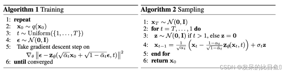
从经验上看，Ho et al. (2020)发现训练扩散模型时，忽略加权项的简化目标效果更好
$$L_t^{\text{simple}}={\mathbb{E}}_{{\mathbf{x}}_0,{\mathbf{z}}_t}[\Vert {\mathbf{z}}_t-{\mathbf{z}}_{\theta }(\sqrt{{\bar{\alpha }}_t}{\mathbf{x}}_0+\sqrt{1-{\bar{\alpha }}_t}{\mathbf{z}}_t,t){\Vert }^2]$$

最后一个简单的目标是
$$L_{\text{simple}}=L_t^{\text{simple}}+C$$

$C$是常数，不依赖于$\theta$

代码

import matplotlib.pyplot as plt
import numpy as np
from sklearn.datasets import make_s_curve
import torch# Setp1. 加载数据
s_curve, _ = make_s_curve(10**4, noise=0.1)
s_curve = s_curve[:,[0, 2]]/10.0## 可视化
fig, ax = plt.subplots()
ax.scatter(*data, color="red", edgecolors="white")
ax.axis("off")dataset = torch.Tensor(s_curve).float()#Step2 确定超参数的值
num_steps = 100 ## 对于步骤， 一开始可以由beta, 分布的均值和标准差来共同决定
#制定每一步的beta
betas = torch.linspace(-6, 6, num_steps) # 返回一个1维张量，包含在区间start和end上均匀间隔的step个点
betas = torch.sigmoid(betas)*(0.5e-2 - 1e-5) + 1e-5## 计算alpha, apha_prod, alpha_prod_previous, alpha_bar_sqrt等变量值
alphas = 1-betas
alphas_prod = torch.cumprod(alphas, 0) # 竖着累积
alphas_prod_p = torch.cat([torch.tensor([1]).float(), alphas_prod[:-1]], 0)
## 保证逆扩散过程也是正态的
alphas_bar_sqrt = torch.sqrt(alphas_prod)
one_minus_alphas_bar_log = torch.log(1-alphas_prod)
one_minus_alphas_bar_sqrt = torch.sqrt(1-alphas_prod)assert alphas.shape==alphas_prod.shape==alphas_prod_p.shape==\
alphas_bar_sqrt.shape==one_minus_alphas_bar_log.shape\
==one_minus_alphas_bar_sqrt.shape
print("all the same shape",betas.shape)#Step3 确定扩散过程任意时刻的采样值
## 公式：
## $q(x_t|x_0) = N(x_t; \sqrt{\bar{a_t}}x_0, \sqrt{1-\bar{a_t}}I)$
# 计算任意时刻x的采样值，基于x_0和重参数化
def q_x(x_0, t):"""可以基于x[0]得到任意时刻t的x[t]"""noise = torch.rand_like(x_0)alphas_t = alphas_bar_sqrt[t]alphas_1_m_t = one_minus_alphas_bar_sqrt[t]return (alphas_t * x_0 + alphas_1_m_t * noise)#在x[0]的基础上添加噪声# Step4 原始数据分布加噪100步后的结果
num_shows = 20
fig,axs = plt.subplots(2,10,figsize=(28,3))
plt.rc('text',color='black')#共有10000个点，每个点包含两个坐标
#生成100步以内每隔5步加噪声后的图像
for i in range(num_shows):j = i//10k = i%10q_i = q_x(dataset,torch.tensor([i*num_steps//num_shows]))#生成t时刻的采样数据axs[j,k].scatter(q_i[:,0],q_i[:,1],color='red',edgecolor='white')axs[j,k].set_axis_off()axs[j,k].set_title('$q(\mathbf{x}_{'+str(i*num_steps//num_shows)+'})$')# Step5 拟合逆扩散过程高斯分布的模型
### 对应$\epsilon_\theta$函数 $\epsilon_\theta(\sqrt{\bar{a_t}}x_0+\sqrt{1-\bar{a_t}}\epsilon, t)$
import torch
import torch.nn as nnclass MLPDiffusion(nn.Module):def __init__(self, n_steps, num_units=128):"""n_steps: 经历多少步num_units: 中间维度"""super().__init__()self.linears = nn.ModuleList([nn.Linear(2, num_units),nn.ReLU(),nn.Linear(num_units, num_units),nn.ReLU(),nn.Linear(num_units, num_units),nn.ReLU(),nn.Linear(num_units,2),])self.step_embeddings = nn.ModuleList([nn.Embedding(n_steps, num_units),nn.Embedding(n_steps, num_units),nn.Embedding(n_steps, num_units),])def forward(self,x,t):
#         x = x_0for idx,embedding_layer in enumerate(self.step_embeddings):t_embedding = embedding_layer(t)x = self.linears[2*idx](x)x += t_embeddingx = self.linears[2*idx+1](x)x = self.linears[-1](x)return x# Step6 训练误差函数
## $L(\theta) = E_{t,x_0,\epsilon[||\epsilon-\epsilon_\theta{(\sqrt{\bar{a_t}}x_0+\sqrt{1-\bar{a_t}}\epsilon, t)}||^2]}$
def diffusion_loss_fn(model, x_0, alphas_bar_sqrt, one_minus_alphas_bar_sqrt, n_steps):"""对任意时刻t进行采样计算loss"""batch_size = x_0.shape[0]#对一个batchsize样本生成随机的时刻t,覆盖到更多不同的tt = torch.randint(0, n_steps, size=(batch_size//2,))t = torch.cat([t, n_steps-1-t], dim=0)t = t.unsqueeze(-1)#x0的系数a = alphas_bar_sqrt[t]#eps的系数aml = one_minus_alphas_bar_sqrt[t]#生成随机噪音epse = torch.randn_like(x_0)#构造模型的输入x = x_0*a+e*aml#送入模型，得到t时刻的随机噪声预测值output = model(x,t.squeeze(-1))#与真实噪声一起计算误差，求平均值return (e - output).square().mean()# Step7 逆扩散采样函数（inference）
"""
在DDPM论文中，作者选择了方案【3】，即让$D_{\theta}$网络的输出等于$\epsilon$，预测噪音法。于是，新的逆向条件分布的均值可以表示成（下式中的$\epsilon$相当于我们定义的广义的$D_{\theta}$网络的具体目标形式）：
p_sample采样的函数是$\mu_\theta{(x_t, t)}=\tilde{\mu}_t(x_t, \frac{1}{\sqrt{\bar{a_t}}}(x_t-\sqrt{1-\bar{a_t}}\epsilon_{\theta}(x_t)))=\frac{1}{\sqrt{a_t}}(x_t-\frac{\beta_t}{\sqrt{1-\bar{a_t}}}\epsilon_{\theta}(x_t, t))$
"""
def p_sample_loop(model, shape, n_steps, betas, ones_minus_alphas_bar_sqrt):"""从x[T]恢复x[T-1]、x[T-2]|...x[0]"""cur_x = torch.randn(shape)x_seq = [cur_x]for i in reversed(range(n_steps)):cur_x = p_sample(model,cur_x,i,betas,one_minus_alphas_bar_sqrt)x_seq.append(cur_x)return x_seqdef p_sample(model, x, t, betas,one_minus_alphas_bar_sqrt):"""从x[T]采样t时刻的重构值"""t = torch.tensor([t])coeff = betas[t] / one_minus_alphas_bar_sqrt[t]eps_theta = model(x, t)mean = (1/(1-betas[t]).sqrt())*(x-(coeff*eps_theta))z = torch.randn_like(x)sigma_t = betas[t].sqrt()sample = mean + sigma_t * zreturn (sample)# Step8 开始训练模型，打印loss及中间重构效果
seed = 1234class EMA():def __init__(self, mu=0.01):self.mu = muself.shadow = {}def register(self, name, val):self.shadow[name] = val.clone()def __call__(self, name, x):assert name in self.shadownew_average = self.mu * x + (1.0-self.mu) * self.shadow[name]self.shadow[name] = new_average.clone()return new_average"""
ema = EMA(0.5)
for name , param in model.named_parameters():if param.requires_grad:ema.register(name, param.data)"""batch_size = 128
dataloader = torch.utils.data.DataLoader(dataset, batch_size=batch_size, shuffle=True)
num_epoch = 4000
plt.rc("text", color="blue")model = MLPDiffusion(num_steps)#输出维度是2，输入是x和step
optimizer = torch.optim.Adam(model.parameters(),lr=1e-3)for t in range(num_epoch):for idx, batch_x in enumerate(dataloader):loss = diffusion_loss_fn(model,batch_x,alphas_bar_sqrt,one_minus_alphas_bar_sqrt,num_steps)optimizer.zero_grad()loss.backward()torch.nn.utils.clip_grad_norm_(model.parameters(), 1.)optimizer.step()if(t%100==0):print(loss)x_seq = p_sample_loop(model, dataset.shape, num_steps, betas, one_minus_alphas_bar_sqrt)fig,axs = plt.subplots(1,10,figsize=(28,3))for i in range(1,11):cur_x = x_seq[i*10].detach()axs[i-1].scatter(cur_x[:,0],cur_x[:,1],color='red',edgecolor='white');axs[i-1].set_axis_off();axs[i-1].set_title('$q(\mathbf{x}_{'+str(i*10)+'})$')

参考

https://lilianweng.github.io/posts/2021-07-11-diffusion-models/