您现在的位置是:主页 > news > 图片网站模版/随州seo
图片网站模版/随州seo
![]() admin2025/5/5 12:25:53【news】
admin2025/5/5 12:25:53【news】
简介图片网站模版,随州seo,p2p网上贷款网站建设方案.docx,西安市城乡建设厅网站本文将介绍利用opencv 和 机器学习相关知识,检测并追踪视频中的车辆。通过将车辆和非车辆的图像进行特征化,并将特征输入分类器,训练出一个分类模型,利用这个分类器提取图片中的车辆特征,剔除误检,得到最终…
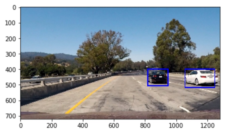
本文将介绍利用opencv 和 机器学习相关知识,检测并追踪视频中的车辆。通过将车辆和非车辆的图像进行特征化,并将特征输入分类器,训练出一个分类模型,利用这个分类器提取图片中的车辆特征,剔除误检,得到最终的检测结果。本文基于python实现,文末留有本文源码和相关材料,读者可以依据本文复现该项目,如有疑问,可留言或私信探讨。
1.整体思路
思路上还是先建立处理单帧图片的方法,然后将该方法应用一张张连续的图片中,即能够实现对视频中车辆的检测。对单张图片的检测过程可归纳如下:
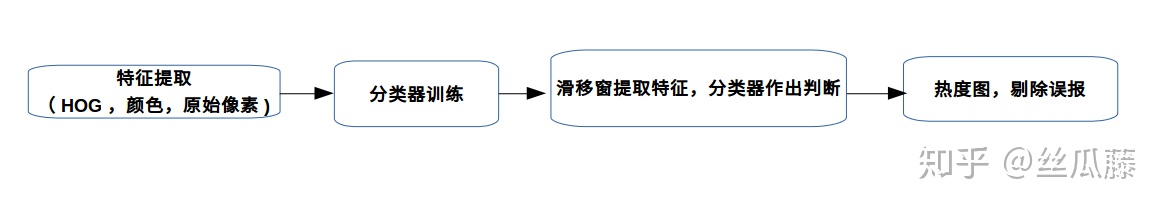
总体来看只有4步,其中前两步是为了判断图像(可能是一个窗口很小的图像)是否是车? 后两步是将这个判断机制应用到一副大的图片上,从图片中提取找到的车。
2. 单张图片的车辆检测
1)导入依赖的工具包
# 导入相关包
2)读取图片
首先我们直观的了解下需要分类的图片特征,观察下“车”和“非车”两个类型的图片,了解数据集的情况。
# 加载图片
car_filename = glob.glob('./vehicles/*/*/*.png')
not_car_filename = glob.glob('./non-vehicles/*/*/*.png')
num_car_image = len(car_filename)
not_car_image = len(not_car_filename)
car_image = mping.imread(car_filename[0])
print('car images: ', num_car_image)
print('not car images: ', not_car_image)
print('Image shape{} and type {}'.format(car_image.shape,car_image.dtype))
通过以上我们得到:
car images数据集中有8792张“车”的图片,8968张“非车”的图片,两种类型的图片数据量大体一致,避免由于数据量偏差造成的模型偏差。图片大小为 64*64 ,3通道。
显示下:
def 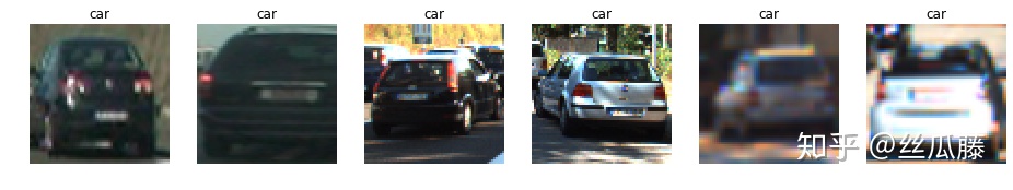

3)特征提取(特征工程)
特征提取的过程简单的理解就是寻找一个“变量”(也可称为特征)来区分“车”和“非车”。通过观察这个“特征”,我们就能分辨出这个图是否是车。
在之前的学习中,我们已经了解到描述一张图片的方式有很多种,例如不同的颜色空间,边缘提取等。本文将采用:HOG(方向梯度直方图)、Color histogram(颜色直方图)、原始像素信息,三个特征结合来区分是否是车。
3.1)HOG 方向梯度直方图
HOG方向梯度直方图就是将图片分割成一个个小方块(block),以每个block中最多的梯度方向作为这个方块的主梯度方向。
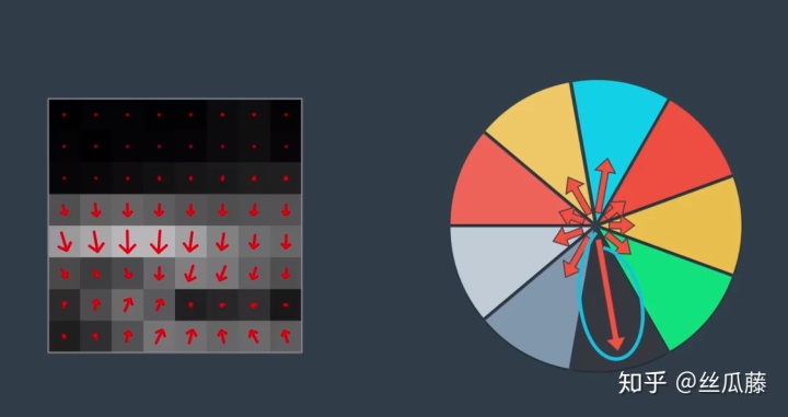
如上图,左侧为一个小方块,里面标出了各个像素点的梯度方向,右边是这个小方块中梯度方向的统计显示,通过计算所有像素梯度的矢量和,得到一个最大的梯度方向,那么就将这个方向作为这个小方块的主梯度方向。换句话说,就是利用这个主梯度方向代表这个block。
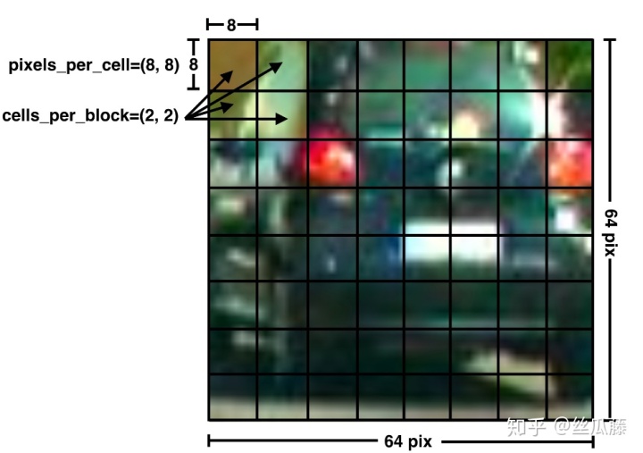
在skimage中有现成的包可以用,使用函数hog可以进行HOG特征提取。该函数的主要参数为:img:图片;orient:梯度的方向个数(一圈360°,分成几个区间);pixels_per_cell:每个cell中的像素点个数;cells_perblock:每个block中的cell数量;transform_sqrt: 是否进行归一化(有利于降低阴影变化的影响);
# 提取HOG特征(方向梯度直方图)
def get_hog_features(img, orient,pix_per_cell, cell_per_block,vis=False, feature_vec =True):if vis == True:features, hog_image = hog(img, orientations=orient, pixels_per_cell=(pix_per_cell, pix_per_cell),cells_per_block=(cell_per_block, cell_per_block), block_norm= 'L2-Hys',transform_sqrt=True, visualise=vis, feature_vector=feature_vec)return features, hog_imageelse:features = hog(img, orientations=orient, pixels_per_cell=(pix_per_cell, pix_per_cell),cells_per_block=(cell_per_block, cell_per_block), block_norm= 'L2-Hys',transform_sqrt=True, visualise=vis, feature_vector=feature_vec)return features
可以直观对比"车”和“非车”图hog特征图的情况:
gray = convert_color(car_image,'Gray')
features,hog_image=get_hog_features(gray, orient = 9, pix_per_cell =8,cell_per_block = 1,vis = True, feature_vec = False)gray = convert_color(noncar_image, 'Gray')
features, hog_image = get_hog_features(gray, orient= 9, pix_per_cell= 8, cell_per_block= 1, vis=True, feature_vec=False)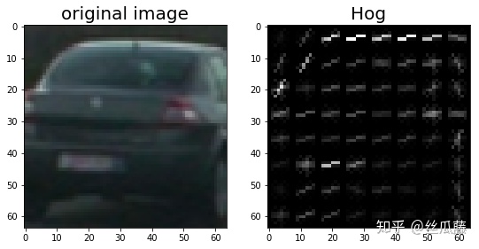
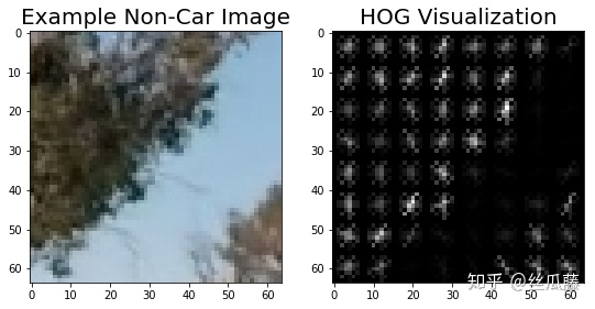
从上面的举例的情况来看,“车”和“非车”图的HOG特征区别还是挺大的。
ps:
关于HOG的相关知识点可以阅读:
1.https://blog.csdn.net/krais_wk/article/details/81119237
2. HOG特征(Histogram of Gradient)学习总结
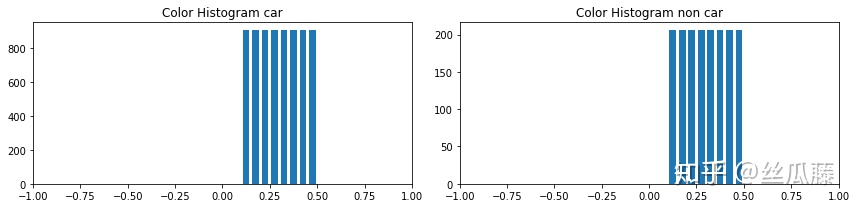
2)颜色直方图
在高级车道线识别的项目中,我们第一次使用了直方图的概念。具体可见其中的第7步:提取车道线:
丝瓜藤:(六)高级车道线识别zhuanlan.zhihu.com
简单的讲,就是统计图像中出现某一规定“数”的次数。在numpy包中有现成的函数histogram可以直接使用:
# 计算颜色histogram
def color_hist(img, nbins=8, bins_range=(0.1,0.5),visualize = False):channel1_hist = np.histogram(img[:,:,0],bins = nbins, range = bins_range)channel2_hist = np.histogram(img[:,:,1],bins = nbins, range = bins_range)channel3_hist = np.histogram(img[:,:,2],bins = nbins, range = bins_range)hist_features = np.concatenate((channel1_hist[0],channel2_hist[0],channel3_hist[0]))    if visualize:bin_edges = channel1_hist[1]bin_centers = (bin_edges[1:]+bin_edges[0:len(bin_edges)-1])/2return hist_features, bin_centersreturn hist_features
np.histogram的参数为:输入图像(一般为单一通道),划分的区间数, 统计的“数”(关注哪个区间的数值)。我们可以对比下“车”和“非车”在0.1和0.5区间内的颜色直方图,分布区别还是很大的。
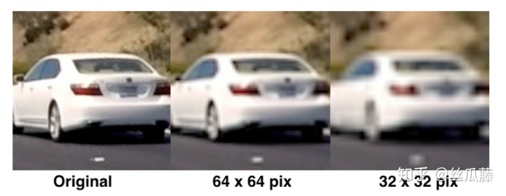
3.3)原始像素信息
“车”和“非车”图片最本质的区别是像素点的区别,但是如果直接把整个像素点都直接输入进去,计算量会非常大,可以考虑改变图像的分辨率。降低分辨率后数据变少,虽然变得模糊,但仍能大体分辨出“车”的形状。
# 原始像素信息
3.4)三种特征结合
将以上三种特征结合,提取图像图像的特征:
def extract_features(image,params,spatial_feat=True, hist_feat=True,hog_feat=True):# 导入参数cspace = params.cspaceorient = params.orientpix_per_cell = params.pix_per_cellcell_per_block = params.cell_per_blockhog_channel = params.hog_channelsize = params.sizehist_bins = params.hist_binshist_range = params.hist_range # 颜色转换feature_image = convert_color(image, cspace) img_features = [] if hog_feat == True:if hog_channel == 'ALL':hog_features = []for channel in range(feature_image.shape[2]):hog_features.append(get_hog_features(feature_image[:,:,channel], orient, pix_per_cell, cell_per_block, vis=False, feature_vec=True))hog_features = np.ravel(hog_features) else:hog_features = get_hog_features(feature_image[:,:,hog_channel],orient,pix_per_cell,cell_per_block,vis = False, feature_vec=True)img_features.append(hog_features)if spatial_feat == True:spatial_features = bin_spatial(feature_image,size)img_features.append(spatial_features)if hist_feat == True:hist_features = color_hist(feature_image,nbins = hist_bins, bins_range = hist_range)img_features.append(hist_features)return np.concatenate(img_features)其中用到了一些子函数:
# 参数类
class FeatureParams():def __init__(self):# HOG parametersself.cspace = 'YCrCb'self.orient = 9self.pix_per_cell = 8self.cell_per_block = 1self.hog_channel = 'ALL'self.size = (8,8)self.hist_bins = 8self.hist_range = (0.1,0.5)
params = FeatureParams()
# 颜色转换函数
def convert_color(image, color_space = 'YCrCb'):if color_space != 'RGB':if color_space == 'HSV':return cv2.cvtColor(image, cv2.COLOR_RGB2HSV)if color_space == 'LUV':return cv2.cvtColor(image, cv2.COLOR_RGB2LUV)elif color_space == 'HLS':return cv2.cvtColor(image, cv2.COLOR_RGB2HLS)elif color_space == 'YUV':return cv2.cvtColor(image, cv2.COLOR_RGB2YUV)elif color_space == 'YCrCb':return cv2.cvtColor(image, cv2.COLOR_RGB2YCrCb)elif color_space == 'Gray':return cv2.cvtColor(image, cv2.COLOR_RGB2GRAY)else: return np.copy(image)4)分类器训练
4.1)数据集准备
准备train data 和 test data数据。sklearn中提供了train_test_split函数从样本中随机按比例分配train data和test data,参数为:所要划分的样本图片,所要划分的样本标签,样本占比,随机数生成的种子。
def split_train_test(car_features, noncar_features):x = np.vstack((car_features, noncar_features)).astype(np.float64)
# car的标签命名为1,not car的标签命名为0y = np.hstack((np.ones(len(car_features)), np.zeros(len(noncar_features))))rand_state = 43x_train,x_test,y_train,y_test = train_test_split(x,y,test_size = 0.2, random_state=rand_state)return x_train,x_test, y_train, y_test
数据还可以进行正则化处理,可以直接使用sklearn中的StandardScaler或RoubstScaler 这是两种正则化方法,这里选择RobustScaler举例。通过正则化后,数据集中的数据特征更加明显,更具有可比性。
def 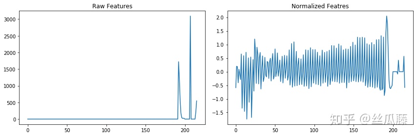
ps:train_test_split 函数可以参考:
sklearn中的train_test_split (随机划分训练集和测试集)www.cnblogs.com4.2)训练模型
在sklearn中已经内置了搭建好的SVM(支持向量机)模型,我们需要做的是调用这个模型,然后利用我们的数据训练这个模型,得到我们自己的模型参数,具体sklearn中SVM的内容和使用方法可以参考:
1.4. Support Vector Machinesscikit-learn.org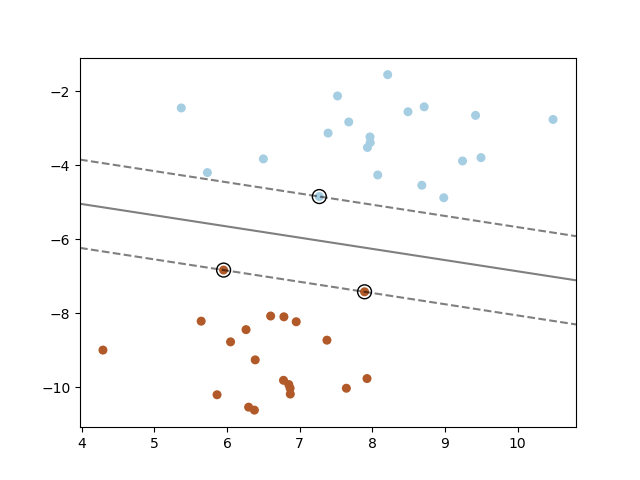
def 调用该函数,训练的结果如下:
13.57 Seconds to train SVC...
Train Accuracy: 0.9665
Test Accuracy: 0.9406
My SVC predicts:  [ 0.  0.  0.  1.  0.  1.  0.  0.  1.  1.]
For these 10 labels:  [ 1.  0.  1.  1.  0.  1.  0.  0.  1.  1.]
0.00363 Seconds to predict 10 labels with SVC
从输出结果来看,模型训练用了13.57s,测试精度为94.06%。通过参数调整能够提高模型的精度,但本文重在整理项目流程和思路,不在调参方面过多纠结,感兴趣的可以进行参数优化。
5)滑移窗提取特征
5.1) 滑动窗口
在高级车道线检测中我们也使用了滑移窗技术,通过一个矩形窗在图片上运动,将图片切割成一个个小的矩形图片。需要注意的是,为了避免漏掉一些特征,相邻的矩形窗之间有重合。
def slide_window(img, x_start_stop=[None, None], y_start_stop=[None, None], xy_window=(64, 64), xy_overlap=(0.85, 0.85)):# 目前定义的相邻两个滑移窗的重合度为85%# 确定滑移窗的边界,如果没有定义边界就以图形的尺寸为最终边界;if x_start_stop[0] == None:x_start_stop[0] = 0if x_start_stop[1] == None:x_start_stop[1] = img.shape[1]if y_start_stop[0] == None:y_start_stop[0] = 0if y_start_stop[1] == None:y_start_stop[1] = img.shape[0]# 计算整个滑移窗边界的大小; xspan = x_start_stop[1] - x_start_stop[0]yspan = y_start_stop[1] - y_start_stop[0]# 计算每移动一步需要移动多少个pix,窗口的大小为xy_windownx_pix_per_step = np.int(xy_window[0]*(1 - xy_overlap[0]))ny_pix_per_step = np.int(xy_window[1]*(1 - xy_overlap[1]))# 计算x和y方向窗口的数量nx_buffer = np.int(xy_window[0]*(xy_overlap[0]))ny_buffer = np.int(xy_window[1]*(xy_overlap[1]))nx_windows = np.int((xspan-nx_buffer)/nx_pix_per_step) ny_windows = np.int((yspan-ny_buffer)/ny_pix_per_step) # I记录窗口的位置window_list = []for ys in range(ny_windows):for xs in range(nx_windows):# Calculate window positionstartx = xs*nx_pix_per_step + x_start_stop[0]endx = startx + xy_window[0]starty = ys*ny_pix_per_step + y_start_stop[0]endy = starty + xy_window[1]window_list.append(((startx, starty), (endx, endy)))# 返回窗口的位置return window_list5.2) 利用分类器判断窗口是否为车
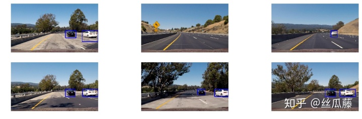
将一个个滑移窗截取到的图片输入到分类器中,然分类器判断是否为车。
def 为了方便观察,我们将识别为车的滑移窗画到图片上:
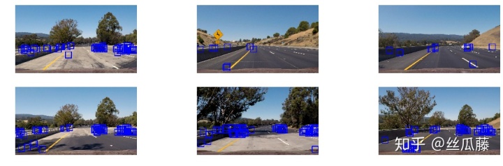
由于滑移窗有一定的重合度,会出现一个车被多个滑移窗检测到的情况,还会出现误检。
除了通过每次移动多少个像素点来进行滑移窗之外,还可以把多个像素点拼成一个块,然后每次移动一个块的一定百分比。这是同一思想的不同实现方法,这里不深入说明,感兴趣可以进行尝试。
仔细观察发现,其实我们这种固定滑移窗大小的搜索方法是有一定缺陷的。车辆在图片中呈现的是“近大远小”,而我们每次都以同样的大小截取图片输入分类器,图片大了之后会给特征向量带来更多的不确定性。
因此我们采用可变大小的方式:在图像上按照由远及近划定区域,不同区域使用不同的比例因子对滑动窗的大小进行缩放。
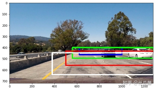
def multi_scale_find_cars(img, svc, scaler, params, return_all=False):# 4个区域分别采用不同大小的比例缩放因子y_start_stops = [[400,464],[400,496],[432,560],[448,644]]x_start_stops = [[620,1000],[560,1280],[500,1280],[380,1280]]car_windows = []for i in range(len(scales)):scale = scales[i]for j in range(2):y_offset = j*16windows = search_windows(img, clf, scaler, params, y_start_stop=[y_start_stops[i][0],y_start_stops[i][1]+y_offset], xy_window=(64, 64), xy_overlap=(0.8, 0.8))car_windows.extend(windows)return np.array(car_windows)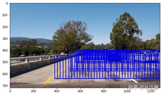
通过这一操作,减少了误识别的情况,但是还是没有解决一个车被多个窗口识别的情况。
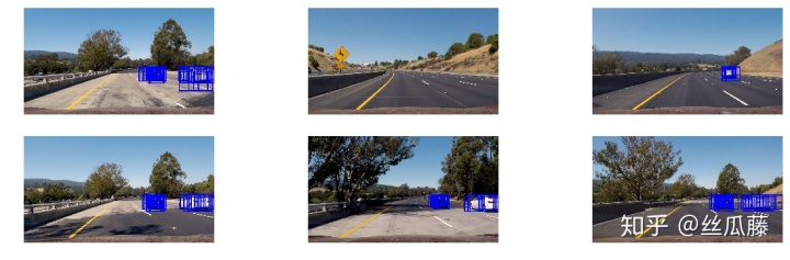
5.3)热度图
被检测到的次数越多,车辆附近出现的矩形框也就越多;可以转换思路理解成“热度图”,被检测到的次数越多,这个区域越“热”。我们可以设定一个阈值,当出现n次检测之后,判断为该区域有车辆,最终输出一个框。
def add_heat(heatmap, bbox_list):for box in bbox_list:# 每出现一个框,热度图加1heatmap[box[0][1]:box[1][1], box[0][0]:box[1][0]] += 1return heatmapdef apply_threshold(heatmap, threshold):# 小于阈值的热度图置0heatmap[heatmap <= threshold] = 0# 返回热度图return heatmap
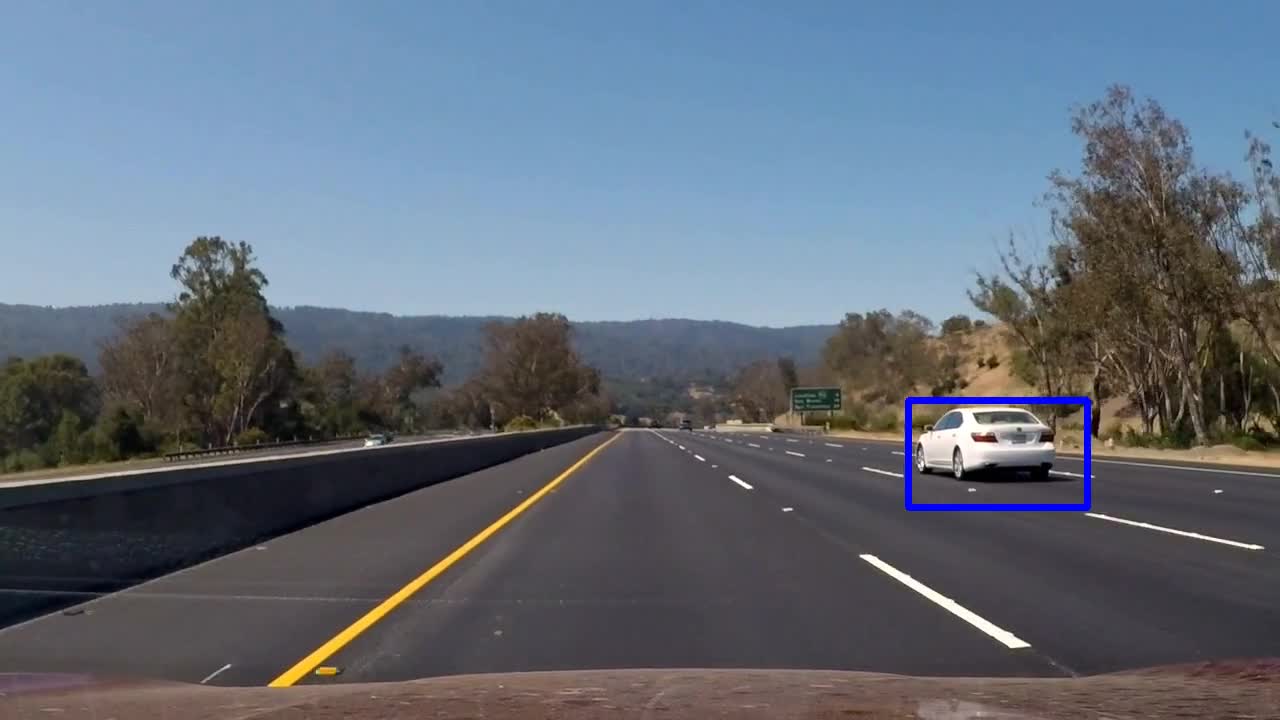
# 画框
def draw_labeled_bboxes(img, labels):for car_number in range(1, labels[1]+1):nonzero = (labels[0] == car_number).nonzero()nonzeroy = np.array(nonzero[0])nonzerox = np.array(nonzero[1])bbox = ((np.min(nonzerox), np.min(nonzeroy)), (np.max(nonzerox), np.max(nonzeroy)))cv2.rectangle(img, bbox[0], bbox[1], (0,0,255), 6)return imgdef draw_labeled_windows(image, boxes, threshold=2):heat = np.zeros_like(image[:,:,0]).astype(np.float)heat = add_heat(heat,boxes) heat = apply_threshold(heat,threshold) heatmap = np.clip(heat, 0, 255)
# 给剩下的热图打标签,相当于统计车的数量 labels = label(heatmap)draw_img = draw_labeled_bboxes(np.copy(image), labels) return heatmap, labels, draw_img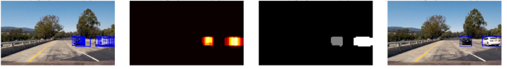
3.视频处理
1)组织检测函数
from collections import deque
def pipeline(image, svc=svc, scaler=scaler, params=params):car_windows = multi_scale_find_cars(image, svc, scaler, params)  _,_,draw_image = draw_labeled_windows(image, car_windows, threshold=2)return draw_image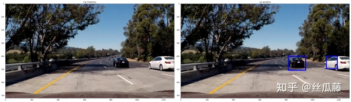
2)视频检测
导入视频的源地址和输出视频的目标地址,调用pipline,处理视频。
def test_video(src_path, dst_path):project_output = dst_path clip1 = VideoFileClip(src_path)white_clip = clip1.fl_image(pipeline)test_video('test_video.mp4','test_videos_output/test_video.mp4')
4. 参考文献
1.本项目来源于Udacity:
Udacitycn.udacity.com
2.HOG特征(Histogram of Gradient)学习总结
3.https://blog.csdn.net/vola9527/article/details/70144811
4.Python3.1-标准库之Numpy - 仙守 - 博客园
5.sklearn GridSearchCV : ValueError: X has 21 features per sample; expecting 19
6.项目相关资料和素材如下,留给有需要的人:
链接:https://pan.baidu.com/s/1aYp3jSmaWVekOX0Md2HScg
提取码:dhwt